|
|
||||||||||||||||||||||||||||||||||||

the authors
|
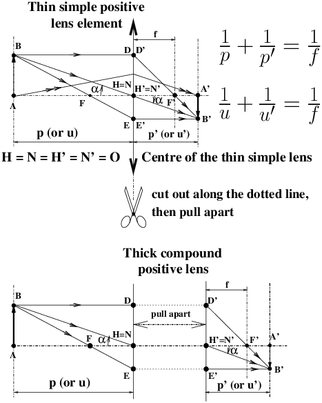
A photographic lens is not a thin simple lens!
| |||||||||||||||||||||||||||||||||||


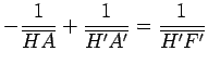
 (1) (1) |
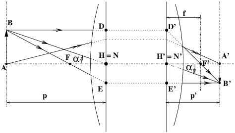
simply measure the distances p and p′ (or u and u′ as written in English textbooks) from the respective principal points: measure p from H (for object space), and p′ from H′ (for image space).
Formula (1) is known in France as Descartes’ Formula, it is written here in its simplified form valid for a positive optical system in which the quantities p and p′ are always considered as positive distances; these are the ones used in photographic practice.
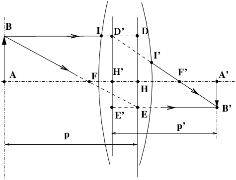
In a wide-angle lens for reflex cameras, the principal image point H′ can be located completely outside the optical system, between the last lens vertex and the focal plane. We will explain later on the interest of having this principal plane H′ which falls completely outside the lens. The inter-nodal distance, gap between H and H′, can be of any length and can even be negative, but it plays a secondary role in photographic applications.
Note, and this gets a bit complicated, that points H and H′ can be located in a “crossed” way with H on the other side of H′ in the direction of light travel (figure 3), we then say that the HH′ gap (noted with a bar on it, it is a algebraic distance) can be positive or negative. In the case of the figure 1 the inter-nocal distance HH′ is positive because H’ is to the right of H, with the conventional direction of light travel from left to right.
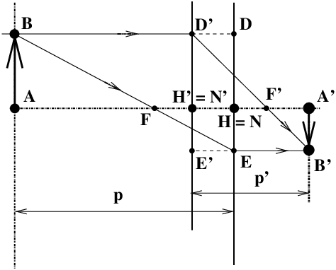
In the case of figure 3, we have HH′ negative, which simply means that H′ is to the left of H; this situation seems a little curious and difficult to understand, but is in fact common (without being an absolute rule), in telephoto lens designs used for all formats when we want the overall length of the lens to be clearly shorter than the focal length. The aim is to reduce the total length and the minimum flange focal distance required in the infinity position. What actually matters in a telephoto lens is that the H′ point is in front of the first lens vertex; the position of the H point is not what matters most.
In the general case, Descartes’ formula (equation (2)) is written with algebraic distances; for example in the case of figure 3: HA < 0 H′A′ > 0 for the formation of images in a photographic lens.
Points A and A′ on the optical axis are on the same vertical line as B and B′, exactly as in the ray tracing and Descartes’ formula for a simple thin lens. The algebraic formulae will be valid in a very general way for all centred systems, even negative systems (for example a tele-converter) and for all positions of objects and images, in the form:
 (2) (2) |
In the general equation (2), the quantity H′F′ is defined as the image focal length of the thick system; for a lens used in air, we have the relation: H′F′=−HF if the input and output media have the same refractive index. It is therefore sufficient to define a single focal length which is positive for a photographic lens, which is a positive optical system and which we shall call for simplicity f; strictly speaking, one should introduce the image focal length f′ and write as follows:
-
H′F′ = f′>0 for a positive system,
-
H′F′ = f′<0 for a negative system.
It is here, looking at figure 3, that a difficulty certainly arises in interpreting the diagram. In fact it is impossible that in this figure incident rays such as BD and BE could actually reach their destination without having been deviated by one of the refracting surfaces constituting the optical system. It should therefore be accepted that the diagram effectively represents only a schematic layout, an assembly of geometric lines that allows the position and size of the image for a given set of source points to be correctly determined.
In figure 4, only the beginning (BI) and the end (I′B′) of the tracings are actually identified with a light path, up to the intersection with of the first refracting surface and then exiting after the last surface; at least if we stick to the slightly inclined rays close to the axis (Gaussian approximation). Most often, the first refracting surface is the surface of the first lens elment (but one can also add a close-up lens or a filter in front of it!); the dotted line is extended until it meets the principal object plane in D, vertical to H. As soon as the last refracting surface has been passed, again a path such as (I′B′) is, as a first approximation, actually followed by light rays (figure 4); the ray seems to come from D′ located vertically to H′. It is nevertheless necessary to slightly modify this vision, which a priori is only valid for slightly inclined rays, very close to the optical axis. If the path of the rays in object space is obviously correct even at very wide angles up to the intersection with the first refracting surface, the symbolic path just after the last surface does not quite correspond to what happens inside a real lens with very tilted rays. Nevertheless, and this is the important point to remember, the symbolic line drawing correctly gives the position and size of the images even with wide-angle lenses (when distortion is small, fish-eye excluded) or with a very large aperture.
Figure 4: The schematic layout of a thick optical system allows to determine where the images are located by means of a symbolic geometrical ray tracing, regardless of the position of the principal planes
This subtle blend between the actual paths actually travelled by light rays and their “dashed” extension to the principal planes is one of the conceptually delicate issues when dealing with geometrical optics applied to thick centred systems. If one accepts the rules, it is as easy as drawing a thin simple lens light beam path.
II 2 Definition of focal lengths
II 2 a) How the thin simple lens helps to define the focal length of any optical system
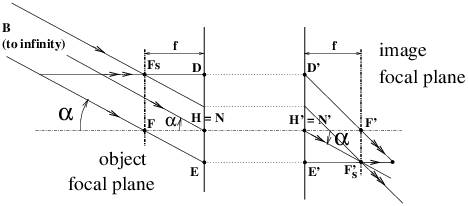
Starting from figure 1, when a beam of light parallel to the axis enters the lens, at the exit the rays converge on the image focal point F′. When an object such as B moves away to the left at a very large distance while keeping constant the angle α between BH and the axis, or – which is equivalent – if a beam of parallel rays making an angle α with the axis enters the lens, these rays intersect on exit at the point Fs′ located at the vertical of F′, i.e. in the image focal plane (figure 5).
Let’s now separate the principal planes H and H′ to get the case of the thick system, the ray tracings in each half space, object and image space behave as in the thin simple lens. By definition we will call focal distance of the thick system the distance H′F′. If we used the lens reversed, in the air as is the rule in current photography, we would find by the same experiment based on the image of a distant object, a distance HF equal to H′F′. There is only one focal length for a system that is used in media with the same refractive index in and out. For a positive system, F′ is located to the right of H′, i.e. the algebraic quantity H′F′ is positive. All photographic lenses are positive systems, but they can be formed from the combination of positive or negative lens groups. Examples of negative optical systems include, in addition to ophthalmic lenses correcting myopia (negative simple lens), the tele-converter used on reflex cameras.
There is therefore a difficulty that arises when trying to estimate the focal length of an unknown thick optical system. The knowledge of this distance conditions the conjugate formulae, and therefore the position and size of the images. Knowledge of the focal length imposes, for example, very strong conditions on the minimum distance between an object and its image on a screen placed at a certain distance supposedly fixed in advance.
If the lens is of a known type and the data sheet is accessible, although you can obviously trust the manufacturer, you will be curious to find out for yourself the values in the data sheet. If the manufacturer indicates that the focal length of the lens is 150.3 mm, one will have very precisely the main H′ plane located 150.3 mm in front of the focus, that is to say approximately 150 mm in front of the image of a very distant object.
II 2 b) How to determine the focal length of a thick system by yourself?
With a simple thin lens, you can focus on the palm of your hand or on a piece of paper the image of a distant object, for example a light bulb placed, say, beyond 50 times the focal length (okay, we’re looking for that focal length! but we can have a rough idea!!). Because the principal points H and H′ are merged in the centre of the thin lens, the distance between the thin lens and the image of this distant object, which is placed at the image focal point F′ gives us a good idea of the focal length. With an unknown thick system, nothing materializes the location of the principal plane H′; if it is possible with a photographic lens to focus the image of a distant object, from which reference point should the quantity H′F′ be measured?
There are professional methods to determine this precisely, but it requires a whole range of instrumentation (collimators, viewfinders, sources, etc.) and an optical bench that the amateur does not have.
Nevertheless it is perfectly possible to estimate the focal length of an unknown thick positive optical system by simple methods.
The first method is a comparison method. It is assumed that you have a 35-mm “film” camera with a lens of known focal length, for example a 50 mm. Open the back of the camera and place a piece of translucent paper on the film rails. Point at two distant objects with good contrast and measure the distance in millimetres on the image. Let’s say we find 20 mm. Let’s form an image of the same scene with the unknown lens, and suppose that we can measure the new distance between the images of the same two objects on a ground glass. For example, this is a view camera lens and we can mount it on the lens panel and focus the image of a distant object on the ground glass. If we find a gap of 60 mm between the images of the two objects with the unknown lens, a very simple proportional correction tells us that the focal length we are looking for is equal to 50x60/20 = 150 mm. This method has the advantage of being totally insensitive to the position of the principal planes, especially for a zoom lens where the principal planes move at the same time the focal length varies.
A second, slightly more precise method applicable to photographic lenses is the following (known in French textbooks as Davanne and Martin’s method [2], figure 6):
-
Locate the image focal point F′ by the image of a distant object, for example a high-contrast landscape element (bell tower [7], dark tree against a sky background). This image will be formed either on a screen or on ground glass. It’s easy with a monorail camera. We will then measure the distance between the last lens vertex (or rather the edge of the lens barrel, or the support plane of the bayonet or lens board, it is better to avoid touching the glass surfaces of a lens with metal objects) and the position of the image. From the position of the last lens vertex, this distance is called back focal distance; the distance between the plane of the bayonet or lens board and this image focal point F′ is called flange focal distance.
Choose a small luminous object of calibrated dimensions, for example a piece of translucent paper with centimetre (or inch) graduations illuminated from behind with a flashlight. Move the screen backwards until an inverted image of this grid is formed which retains the exact dimensions of the object. Having thus “caught” the image the first time, it is now easier to move the object without “losing” this image on the screen, which must be moved while maintaining sharpness. Starting from a position with the object located far away, the image is first formed close to the focal point F′, the transvere magnification is first very small, then by moving the object towards the lens and moving the screen or the viewfinder backwards, point the position for which the grid lines of the image are as exactly as possible equal to 1 cm (or 1 inch), that is to say exactly the same dimension as the centimetric or inch grid used as an object.
The distance by which the screen or ground glass must be moved back between position 1 (infinity-focus) and position 2 (2f-2f) is equal to the focal length.
Figure 6: Approximate determination of the focal length of a thick photographic lens by Davanne and Martin’s method [2]
This method is by far not the most accurate way to determine a focal length, but it will help to become familiar with the minimum distances needed to image objects between the “very far” and the “very near”.
If the lens is turned over or the light is entered from behind, the position of the object focal point F is determined analogously and it can be shown that if the input and output optical media are identical (in our case: air), the two algebraic distances HF and H′F′ are equal and opposite, again by dropping the sign, in arithmetic distances: HF = H′F′ = f. There is, let us repeat, only one focal length for a photographic lens used in the air, and the reversed lens keeps its original focal elength.
There is another method used professionally, called the “nodal point turnstile” ref.[8], [9], which you can use yourself if you are not looking for great precision. It is based on the search for the image stationarity on a screen for a very distant object, ideally located at infinity, when the lens is rotated while keeping the relative positions of the object and the screen fixed (figure 7).
Figure 7: Approximate determination of the focal length of a thick photographic lens using the image nodal point method and the stationary image of an object at infinity; for greater clarity, the entrance and exit refracting surfaces are not shown, and the beam limitation is plotted in a special case where the pupils are placed in the principal planes, a situation close to the reality of quasi-symmetrical view camera lense.

The image of a faraway scene is formed on a screen that is fixed in relation to the landscape so that the object can be considered located at infinity. A professional technician in optical metrology would use a collimator, the amateur would again be content with a far-distant object like the building opposite to his home, or a bell tower.
It is necessary to be able to rotate the lens around any point of the optical axis; this supposes being equipped with a slide, or a monorail view camera reduced to its front standard alone plus a rail, which can be rotated around any vertical axis, adjustable by sliding the rail in relation to the tripod head which imposes this vertical axis of rotation.
The image must be formed on a screen or a ground glass that is detached from the lens, we will try to keep it fixed in relation to the object when turning the lens.
The lens is rotated around a vertical axis in one direction and then in the other; it can be seen that in most cases the image moves in one direction and then in the other, except in a particular position of the rotation axis which corresponds to the image nodal point N′, identical in the air to the principal image point H′.
In reality if we look closely (figure 7) we see that the property of the nodal points to keep the exit angle α′ equal to the input angle α keeps the ray H′F′s parallel to the central entrance ray AH. If the lens has no field curvature, the F′s point after rotation is located a little bit behind the screen. In order to explain this, it is necessary to represent the classical plot by applying the rules but taking into account the fact that the optical axis and the focus F′ have rotated; it is in relation to this new position that the plot must be made. A beam of rays parallel to AH is focused at a point on the focal plane F′s, but since the plane has rotated around H′, the focal point F′s is no longer located exactly on the screen, but a little behind it: the image becomes blurred.
In this “optical turnstile” experiment, even if you rotate correctly around the point H′ = N′, even if at large rotation angles the image remains almost stationary, it becomes a little out of focus. But the important thing is that the exit ray H′F′s remains parallel to the direction of the incident rays. This stationarity property extends closely to the other points of the image, which in turn comes from the focusing of non-parallel rays at AH, making the whole image stationary.
Since the image of the object at infinity is formed in the focal plane passing through F′, the determination of the image nodal point N′ = H′ gives us – by putting the axis of the optical system perpendicular to the screen – the focal length f of the thick system, equal to H′F′.
This property of image stationarity for an object at infinity is the basis for the optical adjustment of moving slit and rotating drum panoramic cameras, for which the image must remain stationary in relation to the film while the lens rotates; these questions will be discussed again in another article.
II 2 c) Minimum distance between the object and its image in a thick optical system
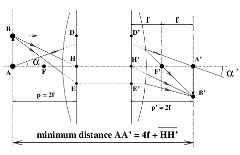
Another question that is quite frequently asked by users of large format cameras with focal lengths that are significantly longer than those of small formats, is: what is the smallest image-object distance Dmini that can be used for focusing? The minimum objet-image distance is obtained in the “2f-2f” position, at magnification -1, and is given by:
| Dmini = 4f + |
| in position “2f-2f” (3) |
If the inter-nodal distance HH′ is small with respect to f as in a thin simple lens, you can see that it takes at least four times the focal length between the object to get a properly focused image. In other words, with a lens of 150 mm focal length (6 inches) for which the inter-nodal distance HH′ is no more than a few mm, you will need at least a distance of 600 mm (24 inches, 2 feet) between the object and the image, and you will need to be able to move the ground glass or film back at least 150 mm beyond the infinity-focus position. In a lens for which the inter-nodal distance HH′ is negative, you will gain a little over this rule, this happens on some telephoto lenses (not all, far from it). But since telephoto lenses are generally long focal lengths, the question of the minimum distance between the object and the image will be more difficult in large format photography than in smaller formats.
In large format photography, very long bellows draw (a very long rail extension for a monorail camera) are quickly needed if one wants to make close-up or macrophoto; most field cameras which do not have a large bellows extension will not allow to easily reach the “2f-2f” position. A notable exception is certain technical cameras with a front folding panel, a typical example of which is the Linhof Technika® , for which the bellows extension allows the “2f-2f” position to be reached in 4x5 inch format with a focal length of 150 mm.
By doing this experiment of finding the location of the image principal plane H′, we will find, according to the optical formula used in the lens, that H′ can be located inside the lens for a quasi-symmetrical standard view camera lens, but that it can be in front of or behind the lens, in the air, respectively in the case of telephoto or retro-focus wide angle lenses for reflex cameras.
III Conclusion
The reading of technical data sheets supplied by lens manufacturers which give the position of the cardinal elements, illustrated by some simple tracings of the optical layout, with the personal handling of thick lenses and the knowledge of the conjugate formulae of thin simple lenses allows to understand without great difficulty the real behaviour of photographic lenses whether they are intended for the 35-mm format, medium format or large format cameras, the rules are the same. After all, the fact that the optics are thick is limited, for the determination of the position and size of the geometric images, to the necessity of taking into account the inter-bodal distance HH′ in the symbolic tracings; even in the somewhat curious cases of telephoto and retro-focus lenses, the difficulty remains modest.
Telephoto lenses and the retro-focus lenses solve some problems related to the back focal distance, but basically nothing changes. As far as the optimisation of these lenses is concerned, imposing a strong constraint on the position of the principal plane H′ relative to the lens design may affect the final performance of the lenses, but all image constructions, magnifications and different settings based on the system’s Gaussian approximation model, with the exception of the inter-nodal HH′ separation, do not differ much from what is well known with a thin simple lens.
We will see in the other articles on https://www.galerie-photo.com how thick optical systems differ from thin simple lenses in questions related to photometry, we will talk about the importance of pupils, then we will finish by presenting the question of slanted congugate planes (Scheimpflug’s rule), and finally we will talk about the questions of diffraction in a thick system.
References
|
All technical terms in this article, which are written in bold,
are explained in this document: |
|
|
(in French, a classical text book on geometrical optics) |
|
|
(in French) Luc Dettwiller, Les instruments d’optique : étude théorique, expérimentale et pratique, ISBN 2-7298-5701-X (Ellipses, Paris, 1997) |
|
|
(in German) Jost Marchesi, Handbuch der Fotografie ISBN 3-9331-3122-7 (Verlag Photographie, Gilching, 1999) |
|
|
By evoking a bell tower as a test object located “optically at infinity”, the author, who lives in Europe, suddenly realises that most the readers of this article do not necessarily have a bell tower nearby, but they will, for sure, find another object in the landscape as an "object at infinity". |
|
|
Moëssard, Paul, « Étude des lentilles et
objectifs photographiques. Première partie. Étude
expérimentale complète d’une lentille ou d’un objectif photographique au
moyen de l’appareil dit “le Tourniquet” »
Gauthier-Villars et fils, Paris, 1889 |
|
|
Searle, G.F.C. 1912 “Revolving Table Method of Measuring
Focal Lengths of Optical Systems” in “Proceedings of the Optical
Convention 1912” pp. 168-171. |
|
|
David Jacobson & John Bercovitz, |
See other articles on https://www.galerie-photo.com
Questions or comments?
-
Send an e-mail to one of the authors
http://bigler.blog.free.fr/public/
images/signature-eb-forums.jpg - Or ask a question on the galerie-photo.info forum (in French, but messages in English are easily understood and answered) http://www.galerie-photo.info/forumgp
Emmanuel Bigler & Yves Colombe 17thFebruary, 2021